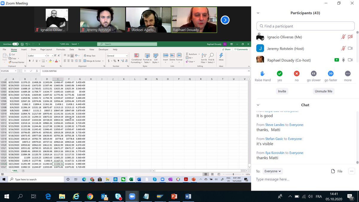
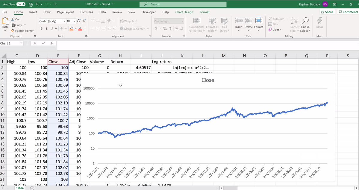
We start with a Yahoo Finance extract of the NASDAQ data from 1971 till today... 2/n

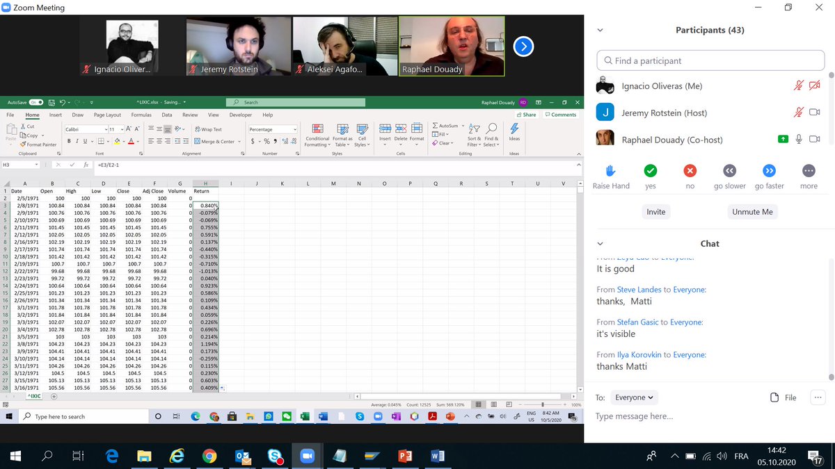
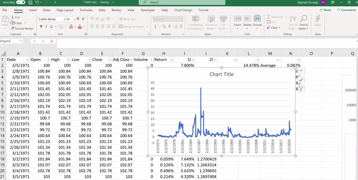
First thing to know about data is integration. We are in the same order of magnitude when we deal with ratios not when we do with differences. The H column stays within the same order of magnitude. Volatility increases, but if we takes the logs-return as in J we re-scale. 3/n

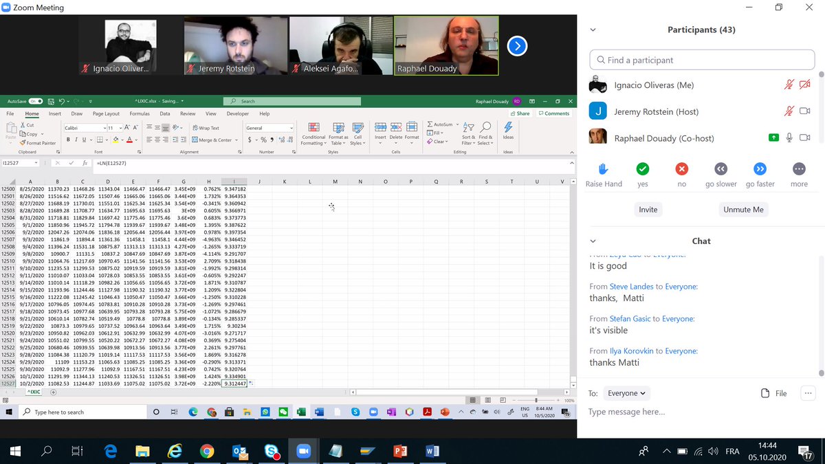
Plotting in log scale. Severe crisis appear now as glitches. Now we can really compare the volatility, and if covid crisis has been worse than 9/11... Lessons: 1) When one deals with time series, it is necessary to re-scale 2) Differentiating the right amount of times... 4/n

Let us look at T-Bills now for a ~15 year period. It appears quite smooth, with rare exceptions, and returns are quite limited. But we are not interested as much in the returns as in the change in those returns: that is our signal. Interest rates are interesting. 5/n

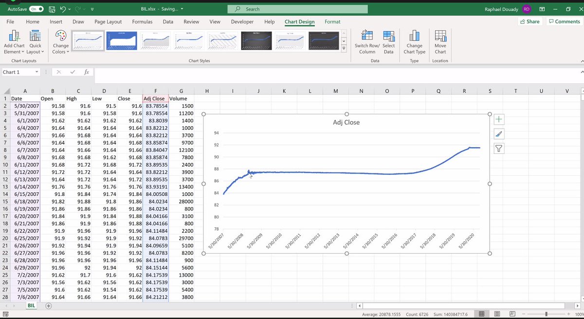
Raphaël tells us how he remembers inflation above 17%, rates at 15%. Bringing these down was very difficult. Q: Is there a link between the scale of the measure, e.g. bi-weekly change vs daily change? Yes, depends on the scale. Look at correlations. . 6/n

You will tell him tomorrow!

If correlations between successive periods are positively correlated, the returns will look smoother. This relates with Madelbrot and Fractal BM... 7/n

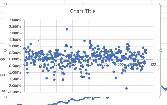
Back to the market plot. No obvious correlation, except when there are "rebounds"... Idea is we get from this course the tools to play with data as kids play with Lego. We need to differentiate sometimes the same way we differentiate velocity from acceleration... 8/n

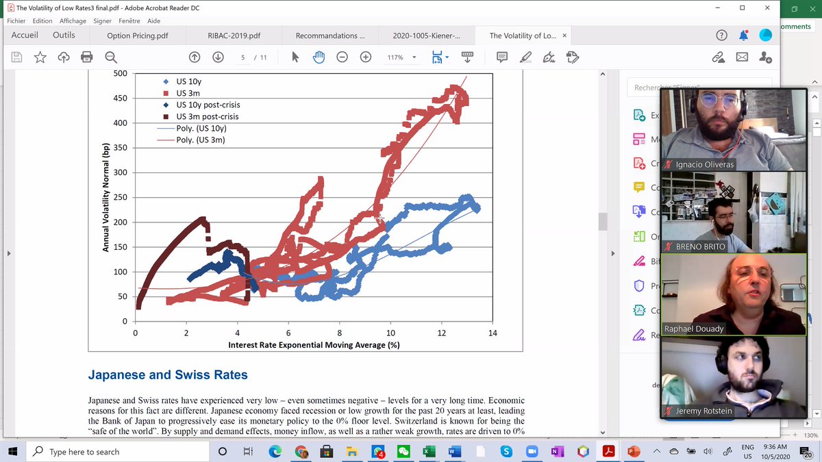
Raphaël shares with us a study he did on interest rates: the higher they go the more volatile they get. This appears true for all countries he studied. The more the rates will grow, the more the volatility of a bond portfolio will rise. But let us go back to the NASDAQ. 9/n

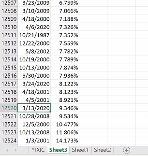
There seems to be 2 sources of Black Swans. One is unexpected events, the second source is accumulated dynamics (bubbles) that don't form in just one day. The largest moves of the stock market are negative (top 5 in the last 50 years). 10/n

I column is std deviation, J ratio of J2 and J3. Log return scales well even with variations like 1987 Black Monday. The Russian Market had a 95% drop in the 90s. Blue plots actual returns, orange log returns. At -100% it goes to infinity, on the upside almost opposite. 11/n

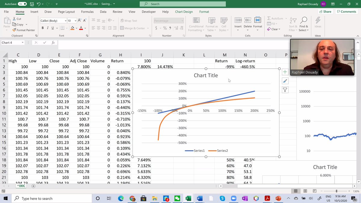
So in the Russian story, if you invested 100 USD you are left with 5 USD. The fuel you need to "rebound" to 100 USD is then massive... 12/n

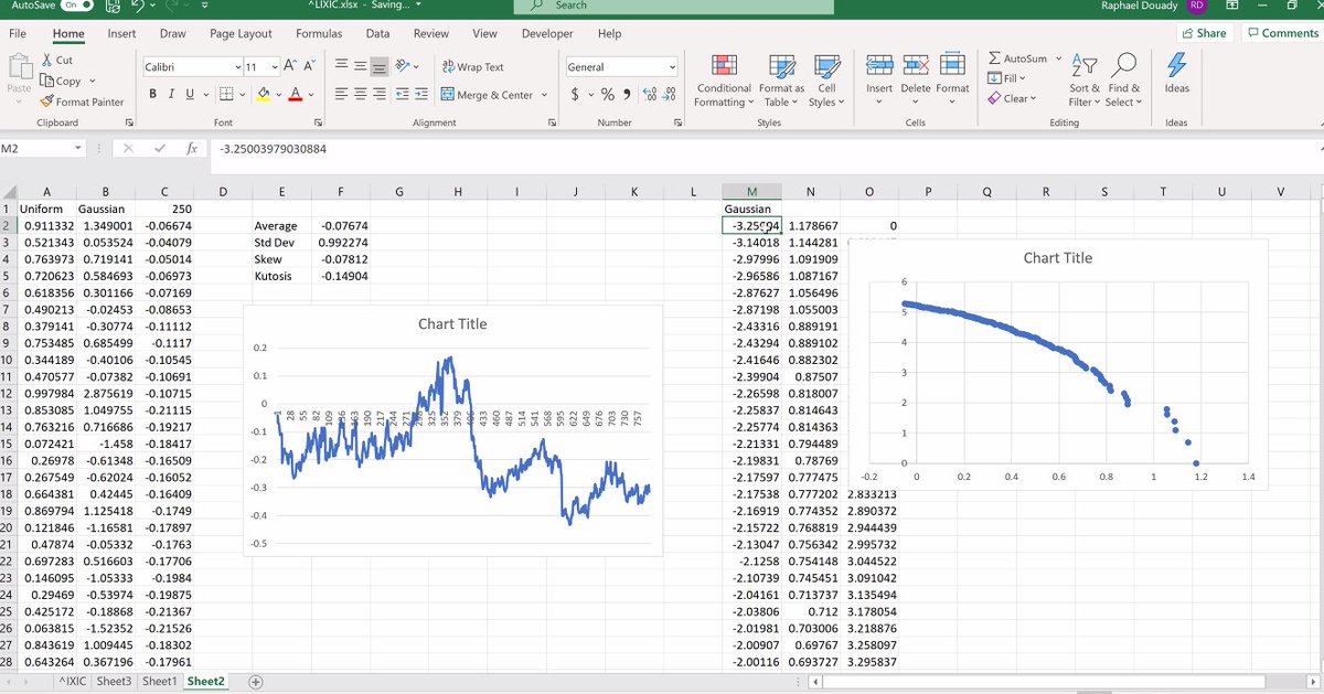
The VC problem can be better grasped by thinking in moments: the cubic (3) of the return on a positive event will dwarf the losses of all other investments that are sterile. Skew corrects it by the variance, kurtosis measure the contribution of one event to the variance... 13/n

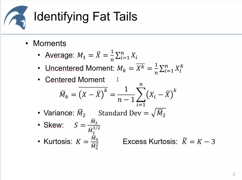
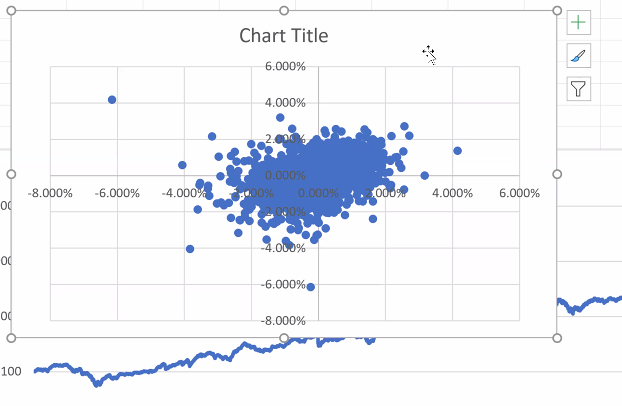
Raphaël plots kurtosis before we will do a short break. @NonMeek asks him how would this look with a normal distribution. Raphaël plays with the data and comes up with the graph in the right. The distribution of the kurtosis is itself skewed, and it often goes negative. 14/n

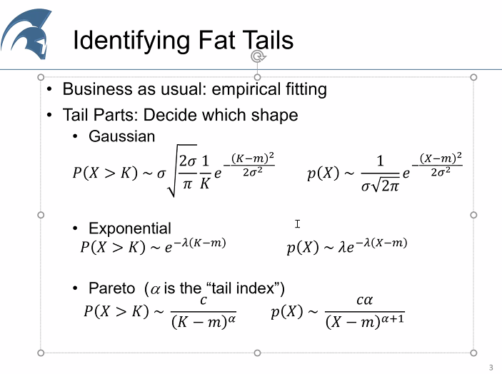
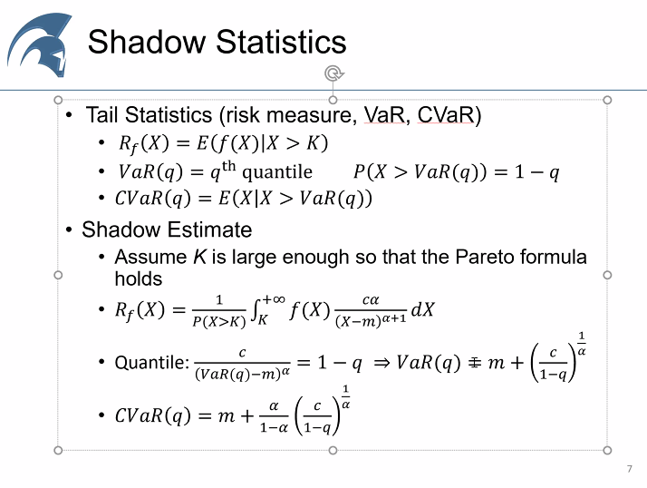
Identifying Fat Tails. Here the distributions we should know, these function explains how the probability decays. NNT found an alpha below 1 when he was studying wars: it is difficult to understand phenomenon with no average. 15/n

Whatever the distribution we can use the Maximum Likelihood Method: we multiply the density of probability and try to find the parameter theta that makes some distribution most probable... 16/n

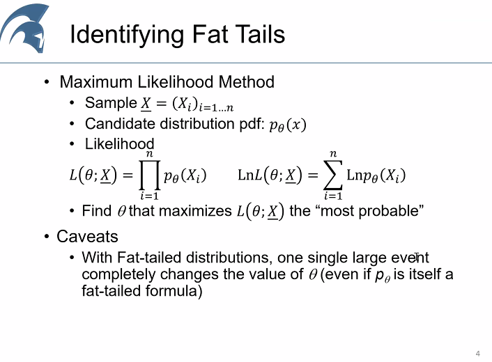
MLE (Maximum Likelihood Estimation) fills tons of books, it is so attractive. But this is tricky: in 99% of the cases we will underestimate (when Bezos is not in our sample) and in 1% of the cases we will vastly overestimate (when he is), so we don't really solve the issue. 17/n

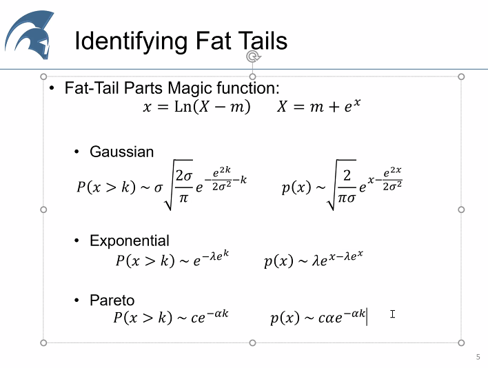
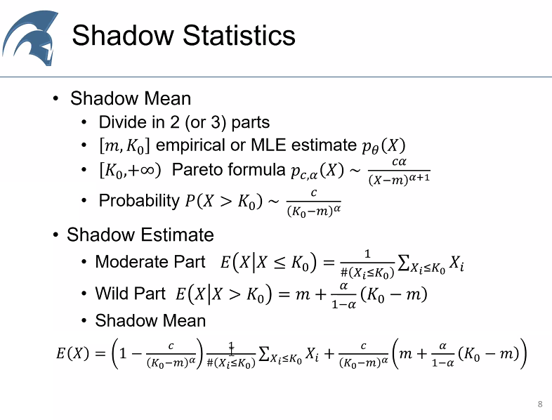
What if we apply the "Fat-Tail Parts Magic function"? This technique would not work well with Gaussian/Exponentials as going to infinity, but works pretty well with the Paretian! 18/n

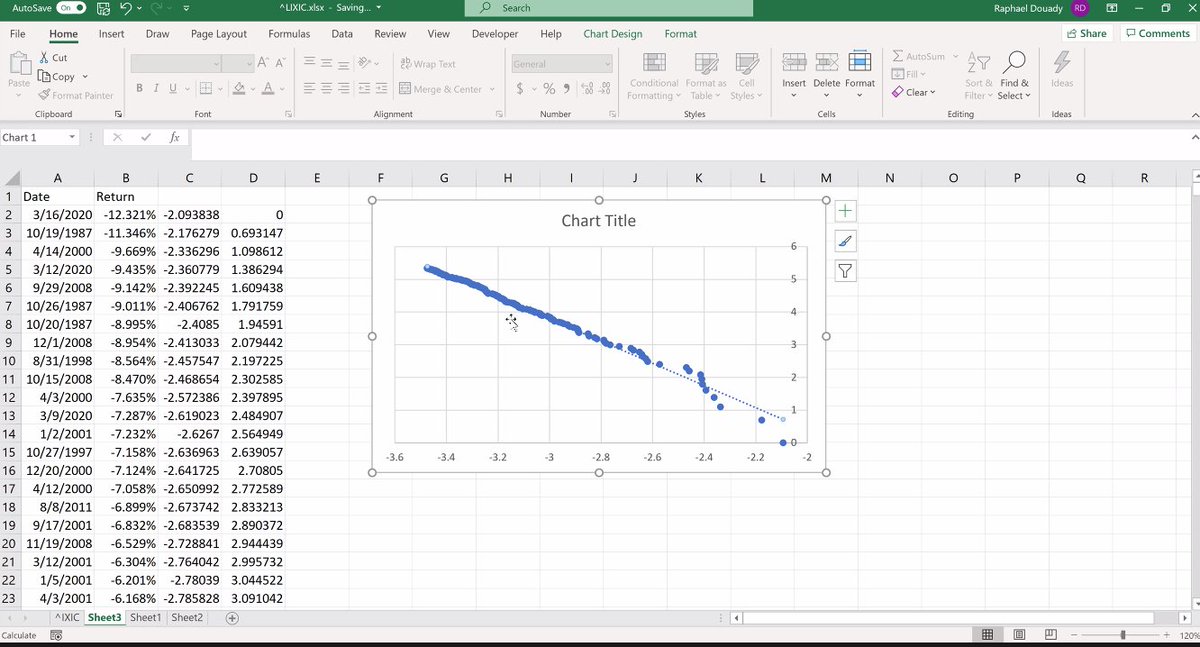
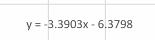
One technique (Tail Index Hill's Estimator): If X is Paretian, P will look as an exponential. Look at the underlined formula: in a way this technique looks like a linear regression... 19/n

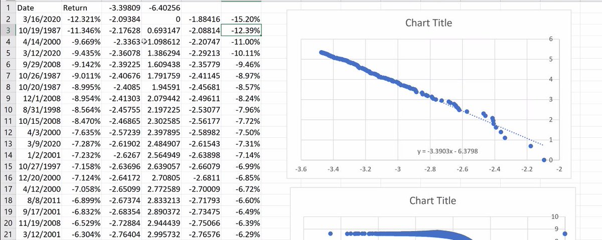
Back to the NASDAQ, the biggest positive days were always rebounds. Raphaël plays with it, gets a nice straight line. We cannot get the same picture when we apply it to the normal distribution. Giving you the estimation of the NASDAQ alpha obtained with this Hill estimator. 20/n

Once we have calculated the alpha, we can analyze the CVaR. Raphaël does so. 21/n

Here the idea is without having Bill Gates in our distribution, anticipating that he exists by the probability distribution. Raphaël invites his friend Patrice Kiener to participate with a presentation on "real life application" of these techniques. 22/n

kappa is the Pareto estimator. If it is below alpha, we have no average, if it is below 2, no variance, if it is below 3 no skew, below 4 no kurtosis... 23/n

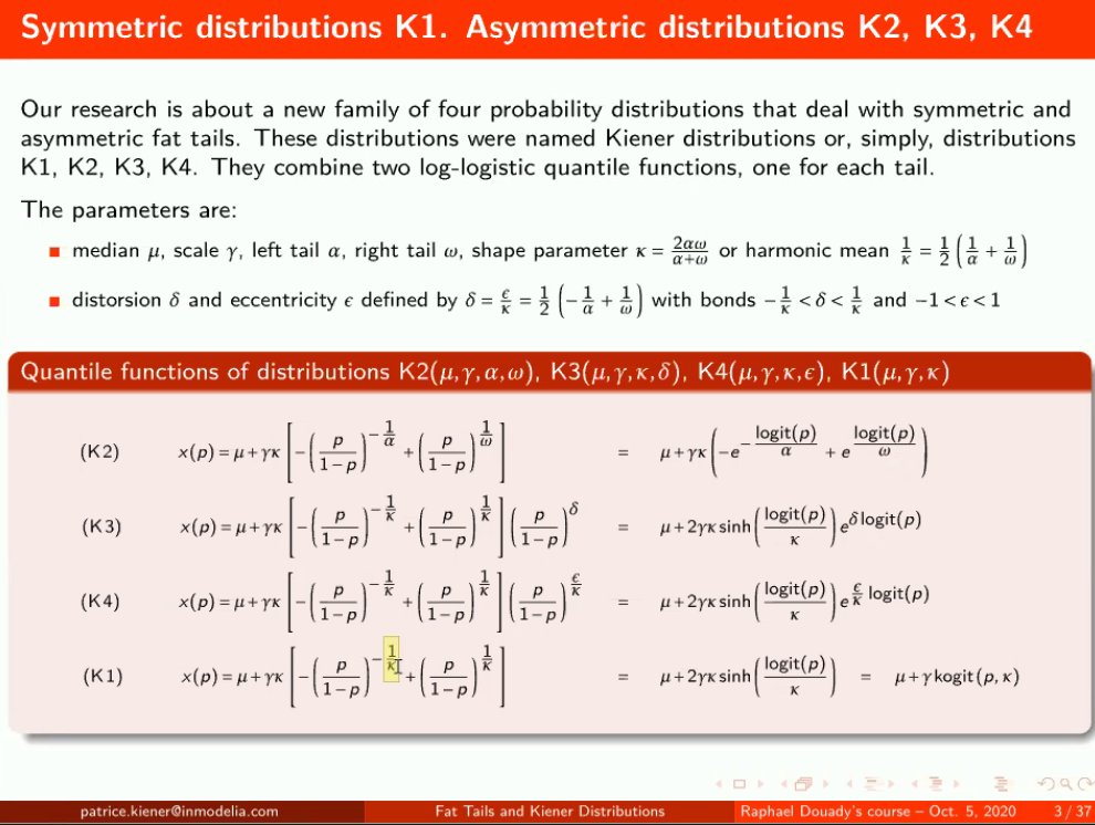
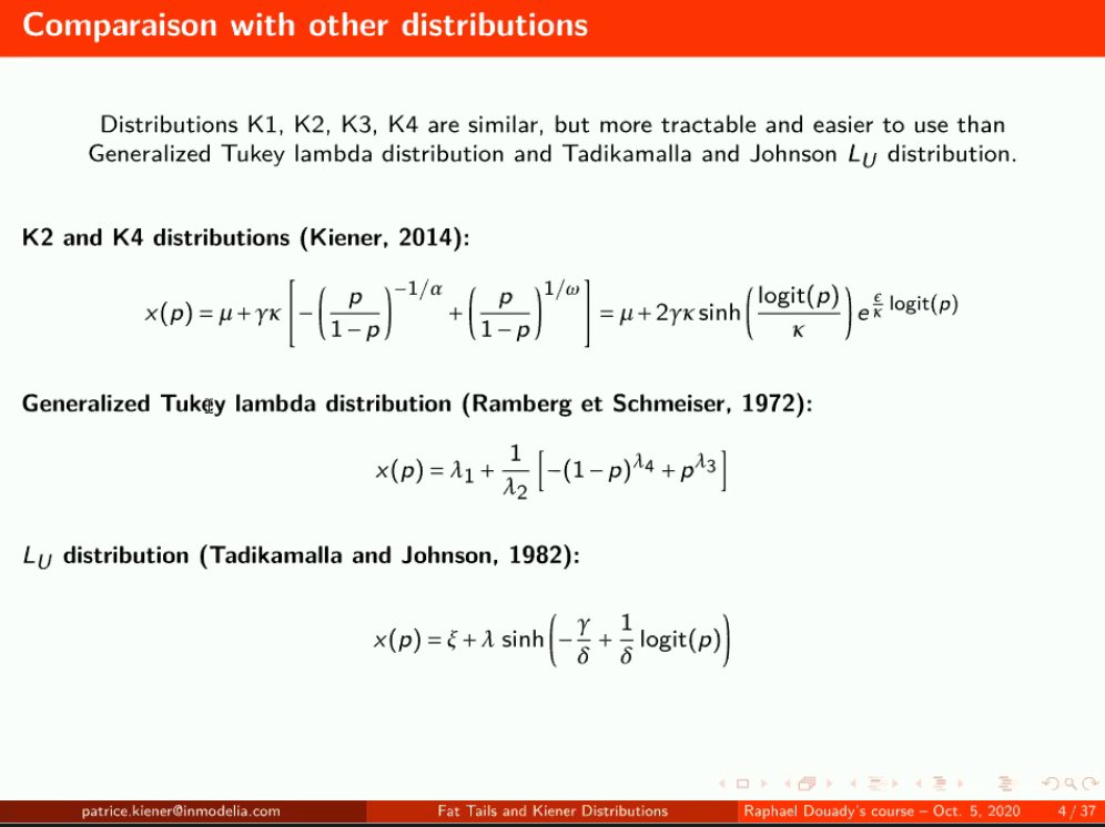
Many people before Patrice and Raphaël has tried to find how to determine a distribution, some examples... 24/n

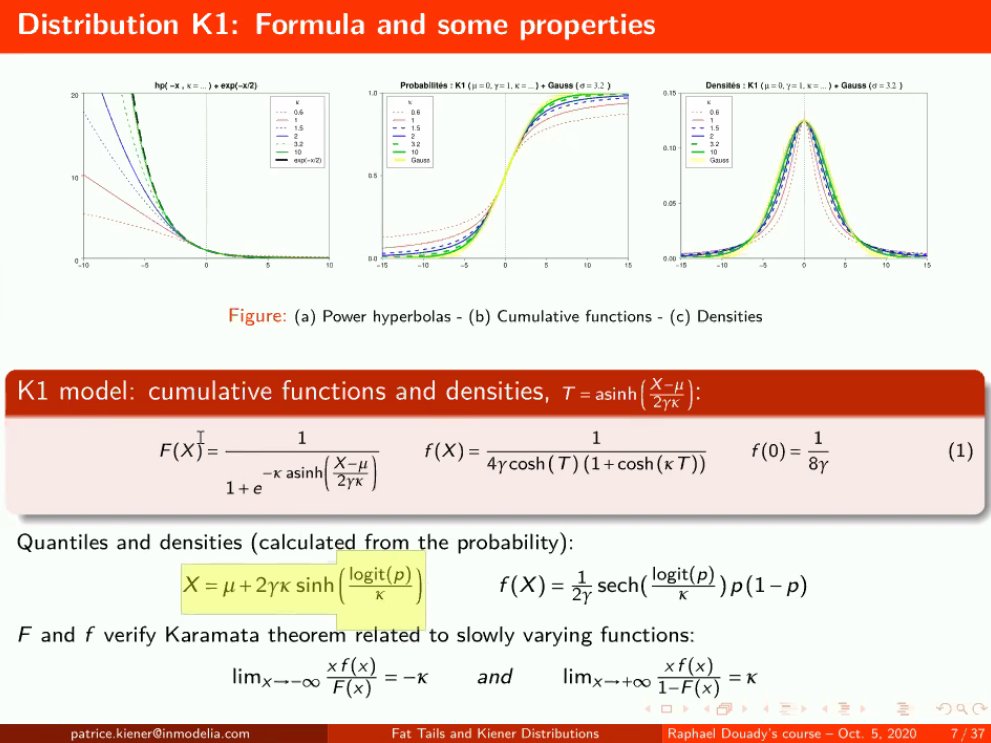
At Raphaël's request, Patrice jumped several slides. Under Fat Tails, we know that the probability denisty in the middle looks thinner as we can observe here... 25/n

I messed up the thread... 26/n

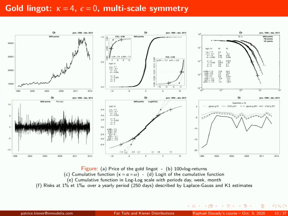
French gold market: very fat tails, kappa/alpha almost 4 and almost no kurtosis. The quantity we will need to cover our investment changes a lot, can double a normal portfolio/Markowitz... 27/n

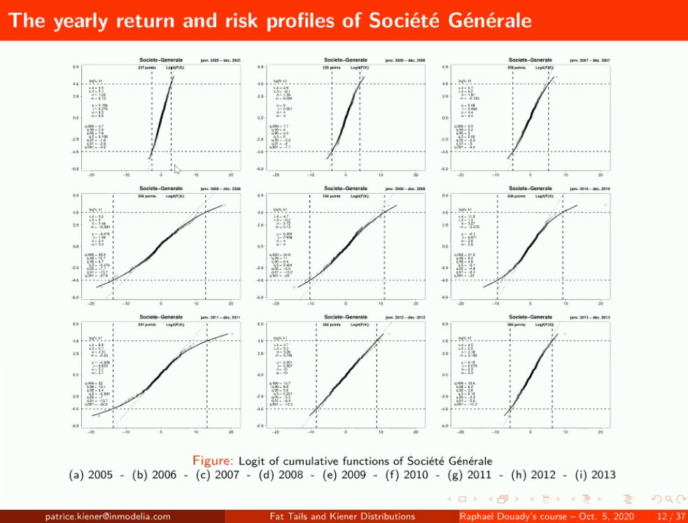
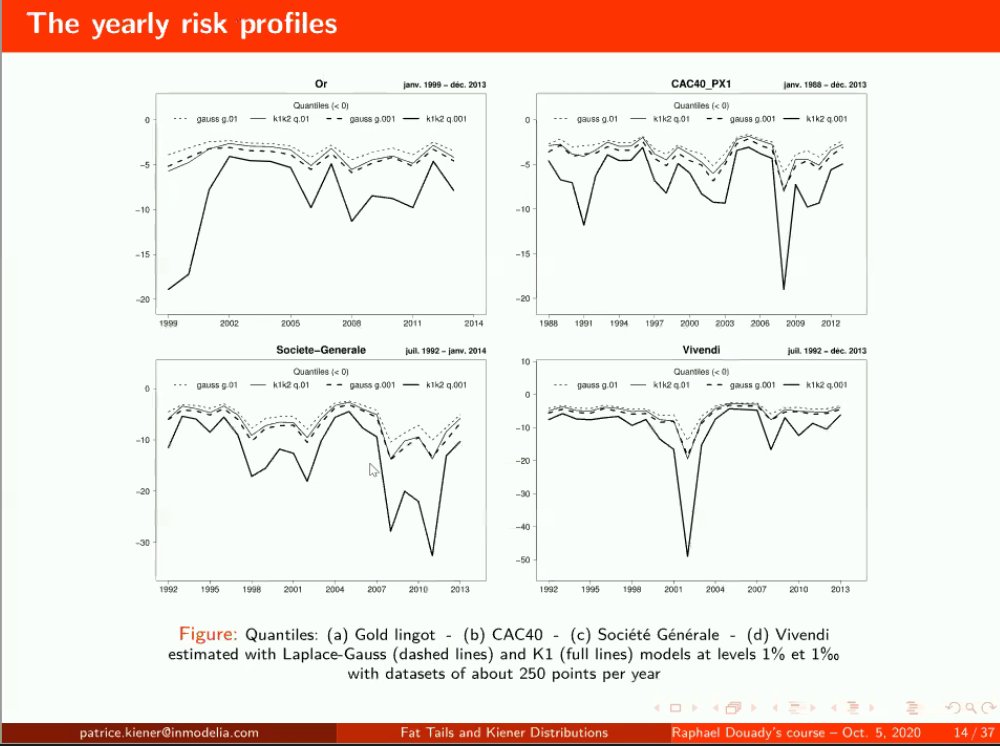
Société Générale had the Kerviel scandal, Vivendi before had a "Messier" scandal as he made the utilities company run out of money with investments in Hollywood. The risk of these in the market and the money needed to cover these positions... 28/n

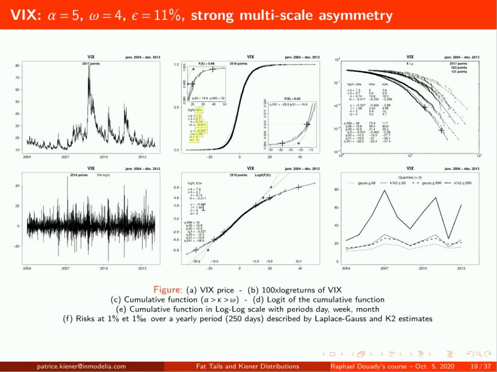
VIX: Fat-Tailed and very asymmetrical. 29/n

Patrice shows as a short clip of the SP500 evolution, Raphaël comments that for the SP500 returns and log returns don't make a big difference. 30/n

Quintile estimation: one manages to do an estimation with 5 data points only. We can estimate the distribution by say knowing what are the values at 99% (and 1%) and 75% (so 25%)... 31/n